2D圖像的三維重建是從一組2D圖像中創(chuàng)建對(duì)象或場(chǎng)景的三維模型的過(guò)程。這個(gè)技術(shù)廣泛應(yīng)用于計(jì)算機(jī)視覺(jué)、機(jī)器人技術(shù)和虛擬現(xiàn)實(shí)等領(lǐng)域。

在本文中，我們將解釋如何使用Python執(zhí)行從2D圖像到三維重建的過(guò)程。我們將使用TempleRing數(shù)據(jù)集作為示例，逐步演示這個(gè)過(guò)程。該數(shù)據(jù)集包含了在對(duì)象周圍的一個(gè)環(huán)上采樣的阿格里真托（Agrigento）“Dioskouroi神廟”復(fù)制品的47個(gè)視圖。

三維重建的關(guān)鍵概念

在深入了解如何使用Python從2D圖像執(zhí)行三維重建的詳細(xì)步驟之前，讓我們首先回顧一些與這個(gè)主題相關(guān)的關(guān)鍵概念。

深度圖

深度圖是一幅圖像，其中每個(gè)像素代表攝像機(jī)和場(chǎng)景中相應(yīng)點(diǎn)之間的距離。深度圖常用于計(jì)算機(jī)視覺(jué)和機(jī)器人技術(shù)中，用于表示場(chǎng)景的三維結(jié)構(gòu)。

有許多不同的方法可以從2D圖像計(jì)算深度圖，包括立體對(duì)應(yīng)、結(jié)構(gòu)光和飛行時(shí)間等。在本文中，我們將使用立體對(duì)應(yīng)來(lái)從示例數(shù)據(jù)集計(jì)算深度圖。

Point Cloud

點(diǎn)云是表示對(duì)象或場(chǎng)景形狀的三維空間中的一組點(diǎn)。點(diǎn)云常用于計(jì)算機(jī)視覺(jué)和機(jī)器人技術(shù)中，用于表示場(chǎng)景的三維結(jié)構(gòu)。

一旦我們計(jì)算出代表場(chǎng)景深度的深度圖，我們可以使用它來(lái)計(jì)算一個(gè)三維點(diǎn)云。這涉及使用有關(guān)攝像機(jī)內(nèi)部和外部參數(shù)的信息，將深度圖中的每個(gè)像素投影回三維空間。

網(wǎng)格

網(wǎng)格是一個(gè)由頂點(diǎn)、邊和面連接而成的表面表示。網(wǎng)格常用于計(jì)算機(jī)圖形學(xué)和虛擬現(xiàn)實(shí)中，用于表示對(duì)象或場(chǎng)景的形狀。

一旦我們計(jì)算出代表對(duì)象或場(chǎng)景形狀的三維點(diǎn)云，我們可以使用它來(lái)生成一個(gè)網(wǎng)格。這涉及使用諸如Marching Cubes或Poisson表面重建等算法，將表面擬合到點(diǎn)云上。

逐步實(shí)現(xiàn)

現(xiàn)在我們已經(jīng)回顧了與2D圖像的三維重建相關(guān)的一些關(guān)鍵概念，讓我們看看如何使用Python執(zhí)行這個(gè)過(guò)程。我們將使用TempleRing數(shù)據(jù)集作為示例，逐步演示這個(gè)過(guò)程。下面是一個(gè)執(zhí)行Temple Ring數(shù)據(jù)集中圖像的三維重建的示例代碼：

安裝庫(kù)：

pip install numpy scipy

導(dǎo)入庫(kù)：

#importing libraries 
import cv2
import numpy as np
import matplotlib.pyplot as plt
import os

加載TempleRing數(shù)據(jù)集的圖像：

# Directory containing the dataset images
dataset_dir = '/content/drive/MyDrive/templeRing'

# Initialize the list to store images
images = []# Attempt to load the grayscale images and store them in the list
for i in range(1, 48):  # Assuming images are named templeR0001.png to templeR0047.png
    img_path = os.path.join(dataset_dir, f'templeR{i:04d}.png')
    img = cv2.imread(img_path, cv2.IMREAD_GRAYSCALE)
    if img is not None:
        images.append(img)
    else:
        print(f"Warning: Unable to load 'templeR{i:04d}.png'")# Visualize the input images
num_rows = 5  # Specify the number of rows
num_cols = 10  # Specify the number of columns
fig, axs = plt.subplots(num_rows, num_cols, figsize=(15, 8))# Loop through the images and display them
for i, img in enumerate(images):
    row_index = i // num_cols  # Calculate the row index for the subplot
    col_index = i % num_cols   # Calculate the column index for the subplot
    axs[row_index, col_index].imshow(img, cmap='gray')
    axs[row_index, col_index].axis('off')# Fill any remaining empty subplots with a white background
for i in range(len(images), num_rows * num_cols):
    row_index = i // num_cols
    col_index = i % num_cols
    axs[row_index, col_index].axis('off')plt.show()

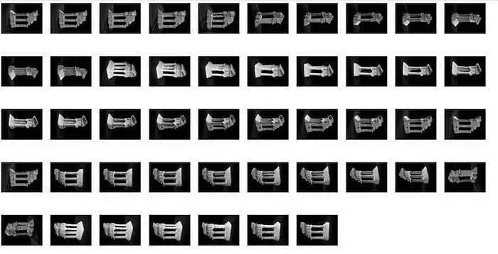
解釋：這段代碼加載灰度圖像序列，將它們排列在網(wǎng)格布局中，并使用matplotlib顯示它們。

為每個(gè)圖像計(jì)算深度圖：

# Directory containing the dataset images
dataset_dir = '/content/drive/MyDrive/templeRing'

# Initialize the list to store images
images = []# Attempt to load the grayscale images and store them in the list
for i in range(1, 48):  # Assuming images are named templeR0001.png to templeR0047.png
    img_path = os.path.join(dataset_dir, f'templeR{i:04d}.png')
    img = cv2.imread(img_path, cv2.IMREAD_GRAYSCALE)
    if img is not None:
        images.append(img)
    else:
        print(f"Warning: Unable to load 'templeR{i:04d}.png'")# Initialize the list to store depth maps
depth_maps = []# Create a StereoBM object with your preferred parameters
stereo = cv2.StereoBM_create(numDisparities=16, blockSize=15)# Loop through the images to calculate depth maps
for img in images:
    # Compute the depth map
    disparity = stereo.compute(img, img)    # Normalize the disparity map for visualization
    disparity_normalized = cv2.normalize(
        disparity, None, 0, 255, cv2.NORM_MINMAX, cv2.CV_8U)    # Append the normalized disparity map to the list of depth maps
    depth_maps.append(disparity_normalized)# Visualize all the depth maps
num_rows = 5  # Specify the number of rows
num_cols = 10  # Specify the number of columns
fig, axs = plt.subplots(num_rows, num_cols, figsize=(15, 8))for i, depth_map in enumerate(depth_maps):
    row_index = i // num_cols  # Calculate the row index for the subplot
    col_index = i % num_cols   # Calculate the column index for the subplot
    axs[row_index, col_index].imshow(depth_map, cmap='jet')
    axs[row_index, col_index].axis('off')# Fill any remaining empty subplots with a white background
for i in range(len(depth_maps), num_rows * num_cols):
    row_index = i // num_cols
    col_index = i % num_cols
    axs[row_index, col_index].axis('off')plt.show()

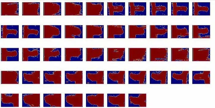
解釋：這段代碼負(fù)責(zé)使用Stereo Block Matching（StereoBM）算法從一系列立體圖像中計(jì)算深度圖。它遍歷灰度立體圖像列表，并為每一對(duì)相鄰圖像計(jì)算深度圖。

可視化每個(gè)圖像的深度圖：

# Initialize an accumulator for the sum of depth maps
sum_depth_map = np.zeros_like(depth_maps[0], dtype=np.float64)

# Compute the sum of all depth maps
for depth_map in depth_maps:
    sum_depth_map += depth_map.astype(np.float64)
# Calculate the mean depth map by dividing the sum by the number of depth maps
mean_depth_map = (sum_depth_map / len(depth_maps)).astype(np.uint8)
# Display the mean depth map
plt.figure(figsize=(8, 6))
plt.imshow(mean_depth_map, cmap='jet')
plt.title('Mean Depth Map')
plt.axis('off')
plt.show()

輸出：

解釋：這段代碼通過(guò)累加深度圖來(lái)計(jì)算平均深度圖。然后，通過(guò)將總和除以深度圖的數(shù)量來(lái)計(jì)算平均值。最后，使用jet顏色圖譜顯示平均深度圖以進(jìn)行可視化。

從平均深度圖計(jì)算三維點(diǎn)云

# Initialize an accumulator for the sum of depth maps
sum_depth_map=np.zeros_like(depth_maps[0],dtype=np.float64)

# Compute the sum of all depth maps
for depth_map in depth_maps:
    sum_depth_map += depth_map.astype(np.float64)# Calculate the mean depth map by dividing the sum by the number of depth maps
mean_depth_map = (sum_depth_map / len(depth_maps)).astype(np.uint8)# Display the mean depth map
plt.figure(figsize=(8, 6))
plt.imshow(mean_depth_map, cmap='jet')
plt.title('Mean Depth Map')
plt.axis('off')
plt.show()

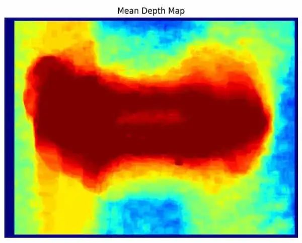
解釋：這段代碼通過(guò)對(duì)深度圖進(jìn)行累加來(lái)計(jì)算平均深度圖。然后，通過(guò)將總和除以深度圖的數(shù)量來(lái)計(jì)算平均值。最后，使用Jet顏色映射來(lái)可視化顯示平均深度圖。

計(jì)算平均深度圖的三維點(diǎn)云

#converting into point cloud 
points_3D = cv2.reprojectImageTo3D(mean_depth_map.astype(np.float32), np.eye(4))

解釋：該代碼將包含點(diǎn)云中點(diǎn)的三維坐標(biāo)，并且您可以使用這些坐標(biāo)進(jìn)行三維重建。

從點(diǎn)云生成網(wǎng)格

安裝庫(kù)

!pip install numpy scipy

導(dǎo)入庫(kù)

#importing libraries 
from scipy.spatial import Delaunay
from skimage import measure
from skimage.measure import marching_cubes

生成網(wǎng)格

verts, faces, normals, values = measure.marching_cubes(points_3D)

解釋：該代碼將Marching Cubes算法應(yīng)用于3D點(diǎn)云以生成網(wǎng)格。它返回定義結(jié)果3D網(wǎng)格的頂點(diǎn)、面、頂點(diǎn)法線和標(biāo)量值。

可視化網(wǎng)格

fig = plt.figure()
ax = fig.add_subplot(111, projection='3d')
ax.plot_trisurf(verts[:, 0], verts[:, 1], verts[:, 2], triangles=faces)
plt.show()

輸出：

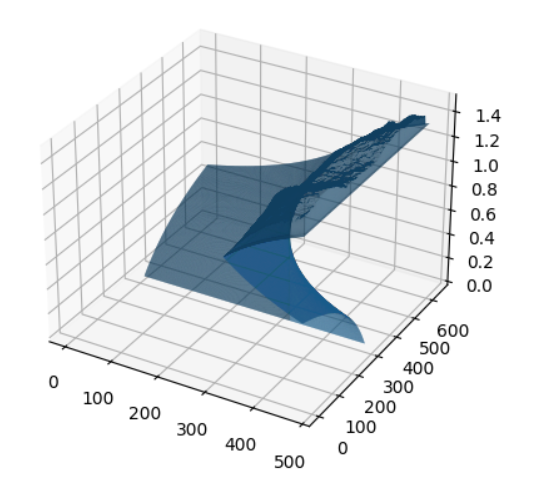
解釋：該代碼使用matplotlib可視化網(wǎng)格。它創(chuàng)建一個(gè)3D圖并使用ax.plot_trisurf方法將網(wǎng)格添加到其中。

這段代碼從Temple Ring數(shù)據(jù)集加載圖像，并使用塊匹配（block matching）進(jìn)行每個(gè)圖像的深度圖計(jì)算，然后通過(guò)平均所有深度圖來(lái)計(jì)算平均深度圖，并使用它來(lái)計(jì)算每個(gè)像素的三維點(diǎn)云。最后，它使用Marching Cubes算法從點(diǎn)云生成網(wǎng)格并進(jìn)行可視化。

結(jié)果比較

# importing the libraries
import matplotlib.pyplot as plt
from mpl_toolkits.mplot3d import Axes3D

# Create a figure with two subplots
fig, axs = plt.subplots(1, 2, figsize=(10, 5))# Visualize the original image in the first subplot
axs[0].imshow(images[0], cmap='gray')
axs[0].axis('off')
axs[0].set_title('Original')# Visualize the reconstructed mesh in the second subplot
ax = fig.add_subplot(1, 2, 2, projection='3d')
ax.plot_trisurf(verts[:, 0], verts[:, 1], verts[:, 2], triangles=faces)
ax.set_title('Reconstructed')# Show the figure
plt.show()

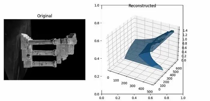
解釋：在此代碼中，使用matplotlib創(chuàng)建了包含兩個(gè)子圖的圖形。在第一個(gè)圖中，顯示了來(lái)自數(shù)據(jù)集的原始圖像。在第二個(gè)圖中，使用3D三角形表面圖可視化了重建的3D網(wǎng)格。

方法2

以下是執(zhí)行來(lái)自TempleRing數(shù)據(jù)集圖像的3D重建的另一個(gè)示例代碼：

引入模塊：

import cv2
import numpy as np
import matplotlib.pyplot as plt
from google.colab.patches import cv2_imshow

加載兩個(gè)Temple Ring數(shù)據(jù)集圖像：

# Load the PNG images (replace with your actual file paths)
image1 = cv2.imread('/content/drive/MyDrive/templeRing/templeR0001.png')
image2 = cv2.imread('/content/drive/MyDrive/templeRing/templeR0002.png'

解釋：該代碼使用OpenCV的cv2.imread函數(shù)從TempleRing數(shù)據(jù)集加載兩個(gè)圖像。

轉(zhuǎn)換為灰度圖：

# Convert images to grayscale
gray1 = cv2.cvtColor(image1, cv2.COLOR_BGR2GRAY)
gray2 = cv2.cvtColor(image2, cv2.COLOR_BGR2GRAY)

該代碼使用OpenCV將兩個(gè)圖像轉(zhuǎn)換為灰度圖像。它們以單通道表示，其中每個(gè)像素的值表示其強(qiáng)度，并且沒(méi)有顏色通道。

查找SIFT關(guān)鍵點(diǎn)和描述符：

# Initialize the SIFT detector
sift = cv2.SIFT_create()

# Detect keypoints and compute descriptors for both images
kp1, des1 = sift.detectAndCompute(gray1, None)
kp2, des2 = sift.detectAndCompute(gray2, None)

該代碼使用尺度不變特征變換（SIFT）算法在兩個(gè)圖像中查找關(guān)鍵點(diǎn)和描述符。它使用OpenCV的cv2.SIFT_create()函數(shù)創(chuàng)建一個(gè)SIFT對(duì)象，并調(diào)用其detectAndCompute方法來(lái)計(jì)算關(guān)鍵點(diǎn)和描述符。

使用FLANN匹配器匹配描述符：

# Create a FLANN-based Matcher object
flann = cv2.FlannBasedMatcher({'algorithm': 0, 'trees': 5}, {})

# Match the descriptors using KNN (k-nearest neighbors)
matches = flann.knnMatch(des1, des2, k=2)

解釋：該代碼使用Fast Library for Approximate Nearest Neighbors（FLANN）匹配器對(duì)描述符進(jìn)行匹配。它使用OpenCV的cv2.FlannBasedMatcher函數(shù)創(chuàng)建FLANN匹配器對(duì)象，并調(diào)用其knnMatch方法來(lái)找到每個(gè)描述符的k個(gè)最近鄰。

使用Lowe的比率測(cè)試篩選出好的匹配項(xiàng)

# Apply Lowe's ratio test to select good matches
good_matches = []
for m, n in matches:
    if m.distance < 0.7 * n.distance:
        good_matches.append(m)

解釋：該代碼使用Lowe的比率測(cè)試篩選出好的匹配項(xiàng)。它使用最近鄰和次近鄰之間距離比的閾值來(lái)確定匹配是否良好。

提取匹配的關(guān)鍵點(diǎn)

# Extract matched keypoints
src_pts = np.float32(
    [kp1[m.queryIdx].pt for m in good_matches]).reshape(-1, 1, 2)
dst_pts = np.float32(
    [kp2[m.trainIdx].pt for m in good_matches]).reshape(-1, 1, 2)

解釋：該代碼從兩組關(guān)鍵點(diǎn)中提取匹配的關(guān)鍵點(diǎn)，這些關(guān)鍵點(diǎn)將用于估算對(duì)齊兩個(gè)圖像的變換。這些關(guān)鍵點(diǎn)的坐標(biāo)存儲(chǔ)在'src_pts'和'dst_pts'中。

使用RANSAC找到單應(yīng)矩陣

# Find the homography matrix using RANSAC
H, _ = cv2.findHomography(src_pts, dst_pts, cv2.RANSAC, 5.0)

在這段代碼中，它使用RANSAC算法基于匹配的關(guān)鍵點(diǎn)計(jì)算描述兩個(gè)圖像之間的變換的單應(yīng)矩陣。單應(yīng)矩陣后來(lái)可以用于拉伸或變換一個(gè)圖像，使其與另一個(gè)圖像對(duì)齊。

使用單應(yīng)矩陣將第一個(gè)圖像進(jìn)行變換

# Perform perspective transformation to warp image1 onto image2
height, width = image2.shape[:2]
result = cv2.warpPerspective(image1, H, (width, height))

# Display the result
cv2_imshow(result)

解釋：該代碼使用單應(yīng)矩陣和OpenCV的cv2.warpPerspective函數(shù)將第一個(gè)圖像進(jìn)行變換。它指定輸出圖像的大小足夠大，可以容納兩個(gè)圖像，然后呈現(xiàn)結(jié)果圖像。

顯示原始圖像和重建圖像

# Display the original images and the reconstructed image side by side
fig, (ax1, ax2, ax3) = plt.subplots(1, 3, figsize=(12, 4))
ax1.imshow(cv2.cvtColor(image1, cv2.COLOR_BGR2RGB))
ax1.set_title('Image 1')
ax1.axis('off')
ax2.imshow(cv2.cvtColor(image2, cv2.COLOR_BGR2RGB))
ax2.set_title('Image 2')
ax2.axis('off')
ax3.imshow(cv2.cvtColor(result, cv2.COLOR_BGR2RGB))
ax3.set_title('Reconstructed Image')
ax3.axis('off')

plt.show()

輸出：

解釋：這段代碼展示了在一個(gè)具有三個(gè)子圖的單一圖形中可視化原始圖像和重建圖像的過(guò)程。它使用matplotlib庫(kù)顯示圖像，并為每個(gè)子圖設(shè)置標(biāo)題和軸屬性。

不同的可能方法

有許多不同的方法和算法可用于從2D圖像執(zhí)行3D重建。選擇的方法取決于諸如輸入圖像的質(zhì)量、攝像機(jī)校準(zhǔn)信息的可用性以及重建的期望準(zhǔn)確性和速度等因素。

一些常見(jiàn)的從2D圖像執(zhí)行3D重建的方法包括立體對(duì)應(yīng)、運(yùn)動(dòng)結(jié)構(gòu)和多視圖立體。每種方法都有其優(yōu)點(diǎn)和缺點(diǎn)，對(duì)于特定應(yīng)用來(lái)說(shuō)，最佳方法取決于具體的要求和約束。

結(jié)論

總的來(lái)說(shuō)，本文概述了使用Python從2D圖像進(jìn)行3D重建的過(guò)程。我們討論了深度圖、點(diǎn)云和網(wǎng)格等關(guān)鍵概念，并使用TempleRing數(shù)據(jù)集演示了使用兩種不同方法逐步進(jìn)行的過(guò)程。我們希望本文能幫助您更好地理解從2D圖像進(jìn)行3D重建以及如何使用Python實(shí)現(xiàn)這一過(guò)程。有許多可用于執(zhí)行3D重建的不同方法和算法，我們鼓勵(lì)您進(jìn)行實(shí)驗(yàn)和探索，以找到最適合您需求的方法。

審核編輯：黃飛